Install, configure, run, and open the report

1. Install

   Use Python 3.10 or newer, create a virtual environment, and install the package in editable mode from the repository root. Link the public Readout 2019 traces so the bundled recipes can locate their data files.

   cd ARCADE
   python -m venv .venv
   source .venv/bin/activate
   pip install -e ".[torch,signature]"
   bash scripts/link_paper_data.sh
   arcade list

   Optional extras unlock method families: torch for neural classifiers, signature for path-signature features, qec for Stim logical-error curves, and dev for tests. A core-only install is pip install -e ..

2. Edit a YAML recipe

   A single configuration file controls the run: the data path and demodulation settings, which classifiers to compare, an optional readout-duration sweep, analytical fabric estimates, and the report output directory. Begin from configs/example.yaml or adapt the reference recipe shown below.

   configs/my_run.yaml · primary settings

   data:
     path: "data/readout2019_adc.h5"
     format: hdf5
     num_qubits: 5
     multiplexed: true
     label_format: joint
     demodulation:
       enabled: true
       frequencies: [64.729e6, 25.366e6, -24.79e6, -70.269e6, -127.282e6]
       sampling_rate: 500.0e6
     split:
       train_ratio: 0.60
       val_ratio: 0.15
       test_ratio: 0.25
       seed: 42
   
   classifiers:
     run:                        # change this list to change the ranking
       - threshold
       - lda
       - qda
       - mlp
       - fnn
       - herqules
   
   sweep:
     enabled: true               # accuracy versus readout duration
     n_points: 8
   
   hardware:
     enabled: true               # analytical lookup tables, DSP, latency
   
   visualization:
     output_dir: ./output/my_run
     format: pdf                 # pdf | html | png

   Validate the configuration before a long run with arcade validate configs/my_run.yaml. For the full published ranking, use configs/paper_all_methods_benchmark.yaml.

3. Run the experiment

   The command-line entry point loads the recipe, prepares traces once, trains every listed method, estimates fabric resources when enabled, and writes plots together with a summary report under visualization.output_dir.

   arcade run configs/my_run.yaml
   # or the reference comparison:
   arcade run configs/paper_all_methods_benchmark.yaml

   The same entry point is available from Python: import arcade; arcade.run("configs/my_run.yaml").

4. Open the report

   After a successful run, open output/…/summary_report.pdf (or the HTML file if you set format: html). The executive summary includes the comparison table, confusion matrices, an optional duration sweep, and a decision block. Later pages add per-method detail.

output/my_run/summary_report.pdf

Report contents

ARCADE Summary Report

Illustrative layout from the five-transmon reference comparison. Your measured values replace these figures after arcade run.

Classifier comparison

Classifier	Accuracy	Infidelity	Five-qubit mean	Per-qubit minimum	Lookup tables	DSP blocks	Latency (ns)
Fully connected network	0.6171	0.3829	0.9074	0.7394	2,499,000	833,000	25.0
Multi-layer perceptron	0.6151	0.3849	0.9070	0.7443	18,560	371	185.0
HERQULES-style	0.6118	0.3882	0.9060	0.7428	2,820	940	20.0
Quadratic discriminant analysis	0.6023	0.3977	0.9032	0.7443	—	1	15.0
Linear discriminant analysis	0.5996	0.4004	0.9024	0.7411	1,600	32	15.0
Next-generation reservoir	0.5976	0.4024	0.9019	0.7410	660	82	165.0
Threshold	0.5776	0.4224	0.8957	0.7427	600	10	10.0

Decision summary

Recommended classifier (joint): fully connected network
Joint accuracy: 0.6171
Five-qubit geometric mean: 0.9074
Near-accuracy lower fabric estimate: HERQULES-style
  (approximately 2,820 lookup tables versus 2,499,000)

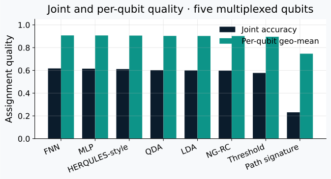
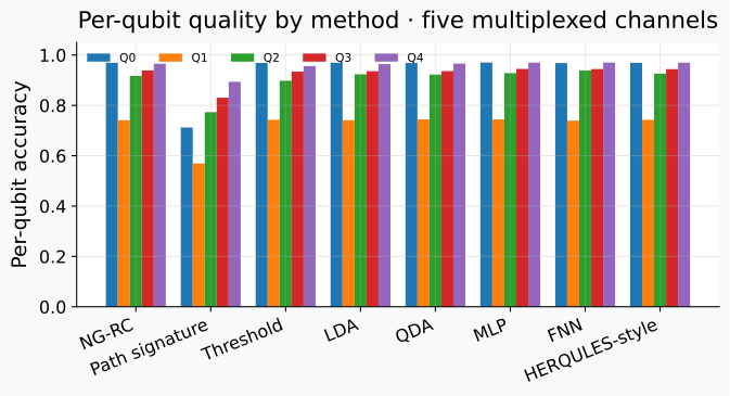
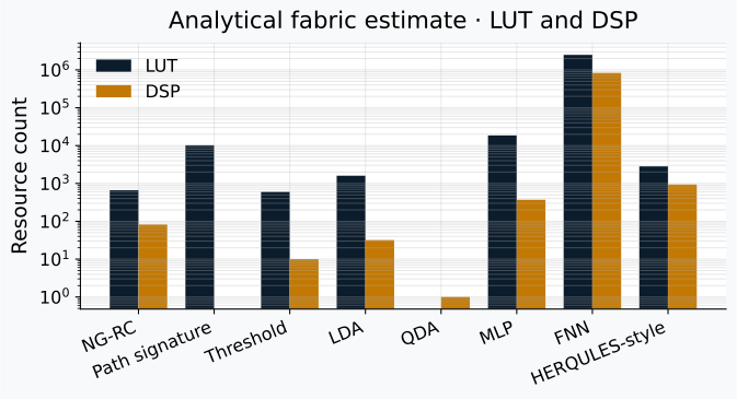
When enabled, the PDF report also includes a confusion-matrix grid, a speed–fidelity sweep overlay, and per-classifier detail pages. Set qec.enabled in the recipe to add logical-error curves; interpret those results on the fault-tolerant quantum computing and near-term goals page.

Bring your own traces

Point data.path at your HDF5 or NumPy recording, set the qubit count, readout frequencies, and label format, then keep the same classifiers.run list. Use a shared recipe for a fair ranking; keep paper-faithful recipes separate when claiming figure parity with a publication.

• Install once. Use an editable package install and linked traces; add optional extras only when needed.
• The recipe is the control surface. Change the method list and feature toggles; keep demodulation and data splits frozen for a fair ranking.
• The report is the deliverable. Accuracy, fabric estimates, and optional duration or quantum-error-correction endings appear in one PDF or HTML file.